- 1. opencv-imgproc
1. opencv-imgproc
imgproc模块包含以下内容:
- 线性和非线性的图像滤波
- 图像几何变换
- 直方图相关
- 结构分析和形状描述
- 运动分析和对象跟踪
- 特征检测
- 目标检测
- ……
1.1. 图像处理
1.1.1. 线性滤波
包括方框滤波、均值滤波、高斯滤波
1.1.1.1. 方框滤波
opencv中,方框滤波封装在函数cv::boxFilter中:
/** @brief Blurs an image using the box filter.

The function smooths an image using the kernel:

\f[\texttt{K} =  \alpha \begin{bmatrix} 1 & 1 & 1 &  \cdots & 1 & 1  \\ 1 & 1 & 1 &  \cdots & 1 & 1  \\ \hdotsfor{6} \\ 1 & 1 & 1 &  \cdots & 1 & 1 \end{bmatrix}\f]

where

\f[\alpha = \begin{cases} \frac{1}{\texttt{ksize.width*ksize.height}} & \texttt{when } \texttt{normalize=true}  \\1 & \texttt{otherwise}\end{cases}\f]

Unnormalized box filter is useful for computing various integral characteristics over each pixel
neighborhood, such as covariance matrices of image derivatives (used in dense optical flow
algorithms, and so on). If you need to compute pixel sums over variable-size windows, use #integral.

@param src input image.
@param dst output image of the same size and type as src.
@param ddepth the output image depth (-1 to use src.depth()).
@param ksize blurring kernel size.
@param anchor anchor point; default value Point(-1,-1) means that the anchor is at the kernel
center.
@param normalize flag, specifying whether the kernel is normalized by its area or not.
@param borderType border mode used to extrapolate pixels outside of the image, see #BorderTypes. #BORDER_WRAP is not supported.
@sa  blur, bilateralFilter, GaussianBlur, medianBlur, integral
 */
CV_EXPORTS_W void boxFilter( InputArray src, OutputArray dst, int ddepth,
                             Size ksize, Point anchor = Point(-1,-1),
                             bool normalize = true,
                             int borderType = BORDER_DEFAULT );
1.1.1.2. 均值滤波
均值滤波是最简单的一种滤波操作,输出图像的每一个像素是滤波核窗口内输入图像对应像素的平均值(所有像素加权平均系数相等)
opencv中,均值滤波封装在函数cv::blur中:
1.1.1.3. 高斯滤波
高斯滤波是一种根据高斯函数的形状选择权值的线性滤波器。
在opencv中,高斯滤波封装在cv::GaussianBlur中。
/** @brief Blurs an image using a Gaussian filter.

The function convolves the source image with the specified Gaussian kernel. In-place filtering is
supported.

@param src input image; the image can have any number of channels, which are processed
independently, but the depth should be CV_8U, CV_16U, CV_16S, CV_32F or CV_64F.
@param dst output image of the same size and type as src.
@param ksize Gaussian kernel size. ksize.width and ksize.height can differ but they both must be
positive and odd. Or, they can be zero's and then they are computed from sigma.
@param sigmaX Gaussian kernel standard deviation in X direction.
@param sigmaY Gaussian kernel standard deviation in Y direction; if sigmaY is zero, it is set to be
equal to sigmaX, if both sigmas are zeros, they are computed from ksize.width and ksize.height,
respectively (see #getGaussianKernel for details); to fully control the result regardless of
possible future modifications of all this semantics, it is recommended to specify all of ksize,
sigmaX, and sigmaY.
@param borderType pixel extrapolation method, see #BorderTypes. #BORDER_WRAP is not supported.

@sa  sepFilter2D, filter2D, blur, boxFilter, bilateralFilter, medianBlur
 */
CV_EXPORTS_W void GaussianBlur( InputArray src, OutputArray dst, Size ksize,
                                double sigmaX, double sigmaY = 0,
                                int borderType = BORDER_DEFAULT );
1.1.2. 非线性滤波
线性滤波可以实现很多不同的图像变换效果,但有的时候,非线性滤波实现的效果更好。
1.1.2.1. 中值滤波
中值滤波是一种典型的非线性滤波技术
- 基本思想:用像素邻域的灰度值的中值来替代该像素点的灰度值
- 优点:可以很好地去除脉冲噪声和高斯噪声,且能保留大部分图像边缘细节
- 弱点:处理时间长
opencv中,中值滤波封装在cv::medianBlur中
/** @brief Blurs an image using the median filter.

The function smoothes an image using the median filter with the \f$\texttt{ksize} \times
\texttt{ksize}\f$ aperture. Each channel of a multi-channel image is processed independently.
In-place operation is supported.

@note The median filter uses #BORDER_REPLICATE internally to cope with border pixels, see #BorderTypes

@param src input 1-, 3-, or 4-channel image; when ksize is 3 or 5, the image depth should be
CV_8U, CV_16U, or CV_32F, for larger aperture sizes, it can only be CV_8U.
@param dst destination array of the same size and type as src.
@param ksize aperture linear size; it must be odd and greater than 1, for example: 3, 5, 7 ...
@sa  bilateralFilter, blur, boxFilter, GaussianBlur
 */
CV_EXPORTS_W void medianBlur( InputArray src, OutputArray dst, int ksize );
1.1.2.2. 双边滤波
1.1.3. 形态学滤波:膨胀和腐蚀
图像处理中的形态学,往往指的是数学形态学。
数学形态学是一门建立在格论和拓扑学基础之上的图像分析学科,是数学形态学图像处理的基本理论,基本的运算包括二值腐蚀和膨胀、二值开闭运算、骨架抽取、极限腐蚀、击中击不中变换、形态学梯度,Top-hat变换、颗粒分析、流域变换、灰值腐蚀和膨胀、灰值开闭运算、灰值形态学梯度等。 膨胀和腐蚀是最基本的形态学操作,主要的作用有:
- 消除噪声
- 分割出独立的图像元素,连接相邻的元素
- 寻找图像中的明显的极大值和极小值区域
- 求出图像的梯度
注意:腐蚀和膨胀是对白色(高亮)部分而言的,不是黑色部分,膨胀是对高亮区域进行扩张。
从数学角度来说,膨胀和腐蚀操作是将图像或图像的一部分(称为A)和核(称为B)进行卷积。
核(kernel)可以是任何形状和大小,它拥有一个单独定义出来的参考点,称为锚点(anchor),多数情况下,核是一个中间带有参考点的正方形或圆形。
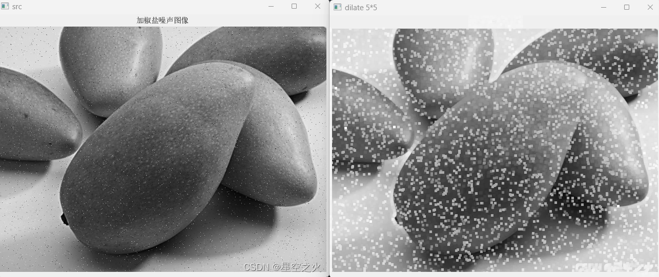
1.1.3.1. 膨胀
膨胀是求局部最大值的操作,即kernel和图像进行卷积,计算kernel覆盖区域的最大值,并把这个最大值赋值给参考点,如此使图像的高亮区域扩张。
在opencv中,膨胀和腐蚀都是调用的morphOP函数:
opencv中,膨胀操作通过cv::dialate函数实现。
/** @brief Dilates an image by using a specific structuring element.
The function dilates the source image using the specified structuring element that determines the
shape of a pixel neighborhood over which the maximum is taken:
\f[\texttt{dst} (x,y) = \max _{(x',y'): \, \texttt{element} (x',y') \ne0 } \texttt{src} (x+x',y+y')\f]
The function supports the in-place mode. Dilation can be applied several ( iterations ) times. In
case of multi-channel images, each channel is processed independently.
@param src input image; the number of channels can be arbitrary, but the depth should be one of
CV_8U, CV_16U, CV_16S, CV_32F or CV_64F.
@param dst output image of the same size and type as src.
@param kernel structuring element used for dilation; if elemenat=Mat(), a 3 x 3 rectangular
structuring element is used. Kernel can be created using #getStructuringElement
@param anchor position of the anchor within the element; default value (-1, -1) means that the
anchor is at the element center.
@param iterations number of times dilation is applied.
@param borderType pixel extrapolation method, see #BorderTypes. #BORDER_WRAP is not suported.
@param borderValue border value in case of a constant border
@sa erode, morphologyEx, getStructuringElement
*/
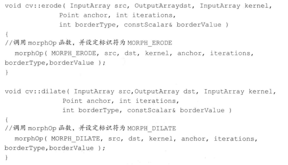
CV_EXPORTS_W void dilate( InputArray src, OutputArray dst, InputArray kernel,
Point anchor = Point(-1,-1), int iterations = 1,
int borderType = BORDER_CONSTANT,
const Scalar& borderValue = morphologyDefaultBorderValue() );
#include<opencv2/opencv.hpp>

using namespace cv;
int main()
{
	Mat src=imread("E:\\test.jpg");
	Mat dilateDst;
	Mat kernel = cv::getStructuringElement(MorphShapes::MORPH_RECT, Size(5, 5));
	cv::dilate(src, dilateDst,kernel);
	imshow("dilate 3*3", dilateDst);
	waitKey(0);
}
效果:
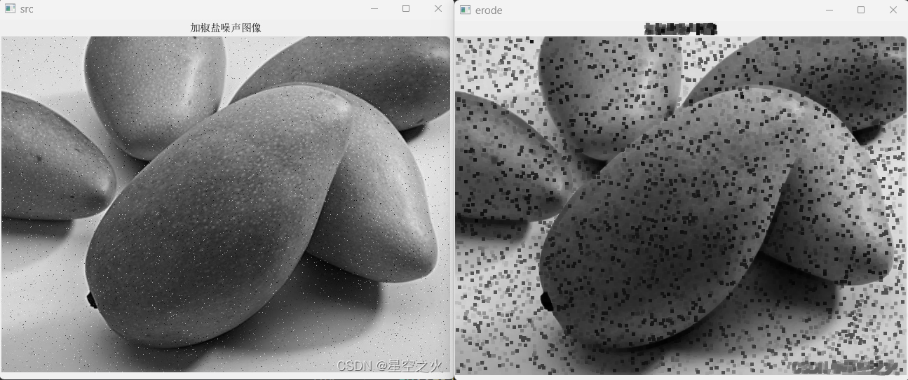
1.1.3.2. 腐蚀
和膨胀相反,腐蚀是求局部最小值的操作。
#include<opencv2/opencv.hpp>

using namespace cv;
int main()
{
	Mat src=imread("E:\\test.jpg");
	Mat dilateDst;
	int n = 5;
	Mat kernel = cv::getStructuringElement(MorphShapes::MORPH_RECT, Size(n, n));
	cv::dilate(src, dilateDst,kernel);
	char wName[50];
	sprintf_s(wName, "dilate %d*%d", n,n);

	imshow("src", src);
	//imshow(wName, dilateDst);
	Mat erodeKernel = getStructuringElement(MorphShapes::MORPH_RECT, Size(n, n));
	Mat erodeDst;
	cv::erode(src, erodeDst, erodeKernel);
	imshow("erode", erodeDst);

	//腐蚀
	waitKey(0);

}
效果:
1.1.3.3. 开运算、闭运算、形态学梯度、顶帽和黑帽
opencv中的morphologyEx函数利用基本的膨胀和腐蚀,来实现更加高级的形态学运算,如开闭运算、形态学梯度、顶帽、黑帽等。
/** @brief Performs advanced morphological transformations.

The function cv::morphologyEx can perform advanced morphological transformations using an erosion and dilation as
basic operations.

Any of the operations can be done in-place. In case of multi-channel images, each channel is
processed independently.

@param src Source image. The number of channels can be arbitrary. The depth should be one of
CV_8U, CV_16U, CV_16S, CV_32F or CV_64F.
@param dst Destination image of the same size and type as source image.
@param op Type of a morphological operation, see #MorphTypes
@param kernel Structuring element. It can be created using #getStructuringElement.
@param anchor Anchor position with the kernel. Negative values mean that the anchor is at the
kernel center.
@param iterations Number of times erosion and dilation are applied.
@param borderType Pixel extrapolation method, see #BorderTypes. #BORDER_WRAP is not supported.
@param borderValue Border value in case of a constant border. The default value has a special
meaning.
@sa  dilate, erode, getStructuringElement
@note The number of iterations is the number of times erosion or dilatation operation will be applied.
For instance, an opening operation (#MORPH_OPEN) with two iterations is equivalent to apply
successively: erode -> erode -> dilate -> dilate (and not erode -> dilate -> erode -> dilate).
 */
CV_EXPORTS_W void morphologyEx( InputArray src, OutputArray dst,
                                int op, InputArray kernel,
                                Point anchor = Point(-1,-1), int iterations = 1,
                                int borderType = BORDER_CONSTANT,
                                const Scalar& borderValue = morphologyDefaultBorderValue() );
1.1.3.3.1. 开运算
先腐蚀后膨胀的过程
1.1.3.3.2. 闭运算:先膨胀后腐蚀的过程。
1.1.3.3.3. 形态学梯度
膨胀图和腐蚀图的差,数学表达式如下:
dst=grad(src,element)=dilate(src,element)-erode(src,element)
1.1.3.3.4. 顶帽运算(top hat)
原图和开运算图像之差
dst=tophat(src,element)=src-open(src,element)
1.1.3.3.5. 黑帽运算(black hat)
闭运算图像和原图之差
dst=blackhat(src,element)=close(src,element)-src
1.1.4. 填充算法-漫水填充
漫水填充法是一种用特定的颜色填充连通区域,经常被用来标记或者分离图像的一部分以便对其进行进一步处理和分析。
opencv中,漫水填充算法由floodFill函数实现,作用是从某个指定的点(种子)开始用特定的颜色填充一个连通域
。
opencv2版本有两个c++重写的floodFill版本:
CV_EXPORTS_W int floodFill( InputOutputArray image, InputOutputArray mask,
                            Point seedPoint, Scalar newVal, CV_OUT Rect* rect=0,
                            Scalar loDiff = Scalar(), Scalar upDiff = Scalar(),
                            int flags = 4 );

/** @example samples/cpp/ffilldemo.cpp
An example using the FloodFill technique
*/

/** @overload

variant without `mask` parameter
*/
CV_EXPORTS int floodFill( InputOutputArray image,
                          Point seedPoint, Scalar newVal, CV_OUT Rect* rect = 0,
                          Scalar loDiff = Scalar(), Scalar upDiff = Scalar(),
                          int flags = 4 );
参数详解:
- image:输入图像
- mask:第二个版本的floodFill独有参数,表示操作的掩膜。它应该是一个单通道的8bit图像且宽、高都比image多2个像素。注意:不会填充mask的非零像素区域。比如,边缘检测算子的输出可以用来作为mask以防止填充到边缘。
- seedPoint:填充的起点
Scalar newVal:像素点被填充的灰度值Rect* rect:默认值0,用于设置floodFill要重绘区域的最小边界矩形区域。Scalar loDiff:默认值Scalar(),表示当前观察像素和邻域像素或者种子像素的亮度或者颜色的最大负差Scalar hiDiff:默认值Scalar(),表示当前观察像素和邻域像素或者种子像素的亮度或者颜色的最大正差int flags:操作标志符,包含三个部分:- 低8位(0-7):控制连通性,设置为4或者8,来决定填充考虑4邻域或者8邻域
- 高8位(16-23):可以为0或者以下两种选项标识符的组合:
- FLOODFILL_FIXED_RANGE:考虑当前像素和种子像素的差,否则考虑当前像素和邻域像素的差。
- FLOODFILL_MASK_ONLY:如果设置,则函数不会填充改变原始图像,即忽略参数newVal,而是去填充mask
- 中间8位:当设置 FLOODFILL_MASK_ONLY时,中间8位的值用来指定mask填充的灰度值,如果中间8位的值为0,则掩码会用1填充。 所有的flags可以用OR操作符连接,比如:使用8邻域填充,且填充固定像素值范围,填充mask而不是源图像,设置填充值为40,则flags设置为: flags=8 | FloodFILL_MASK_ONLY | FLOODFILL_FIXED_RANGE | (40«8)
1.1.5. 图像金字塔与图像缩放
这一节主要讲opencv中的pyrUp和pyrDown进行向下和向上采样,以及专门用于图像尺寸缩放的resize函数
在opencv中对图像缩放主要有两种方式:
resize函数pyrUp和pryDown函数进行向上和向上采样。
说明:resize在improc的Geometric Image transformations子模块,而pyrUp和pyrDown是在imgproc的Image Filtering子模块里。
1.1.5.1. 图像金字塔
图像金字塔是图像多表达中的一种,主要用于图像分割,是一种以多分辨率来解释图像的有效但概念简单的结构。
图像金字塔最初用于机器人视觉和图像压缩,一幅图像的金字塔是一系列以金字塔形状排列的,分辨率逐步降低且来源于同一张原始图的图像集合,其通过梯次向下采样获得,直到达到某个终止条件才停止采样。
金字塔的底部是待处理图像的高分辨率表示,而顶部是低分辨率的近似,层级越高,图像越小,分辨率越低。
1.1.5.1.1. 金字塔分类
- 高斯金字塔(Gaussianpyramid):向下采样,主要的图像金字塔
- 拉普拉斯金字塔(Laplacianpyramid):用来从金字塔低层图像重建上层未采样图像,在数字图像处理中也就是预测残差,可以对图像进行最大程度的还原,配合高斯金字塔一起使用。
两者的主要区别:高斯金字塔用来向下降采样图像,拉普拉斯金字塔用来从金字塔底层图像中向上采样,重建一个图像。
1.1.5.1.2. 生成金字塔过程
从金字塔第i层生成第i+1层(Gi+1),要先用高斯核对Gi进行卷积,然后删除所有的偶数行和偶数列,得到图像面积会变为源图像的1/4,按上述过程对输入图像G0执行操作就可以产生出整个金字塔。
在Opencv中,从金字塔中上一级图像生成下一级图像的可以用PryDown,而PryUp将现有的图像的每个维度都放大两遍。
注意:PryDown和PryUp不是互逆的,即PryUp不是降采样的逆操作,PryUp首先在每个维度上扩大为原来的两倍,新增的行(偶数行)以0填充,然后给指定的滤波器进行卷积去估计丢失像素的近似值。
1.1.5.1.3. 高斯金字塔
高斯金字塔是通过高斯平滑(Gaussian Blur)和亚采样获得一系列下采样图像,也就是说第K层高斯金字塔通过平滑、亚采样就可以获得第K+1层高斯图像。高斯金字塔包含了一系列低通滤波器,其截止频率从上一层到下一层以因子2逐渐增加。
1.1.5.1.4. 拉普拉斯金字塔
Li=Gi-PyrUp(Gi+1)
拉普拉斯金字塔的某一层Li是通过Gi和Gi先缩小后放大的图像的相减得到的。
1.1.5.1.5. 图像金字塔的应用
主要用于图像分割,在图像分割中,先建立一个图像金字塔,然后对Gi和Gi+1的像素直接按照对应的关系建立起父子关系,快速的最初分割可以在金字塔的高层的低分辨率图像上进行,然后逐层对分割加以优化。
1.1.5.1.6. PyrDown和PyrUp
- pyrUp函数
向上采样并模糊一张图像
 CV_EXPORTS_W void pyrUp( InputArray src, OutputArray dst,
                      const Size& dstsize = Size(), int borderType = BORDER_DEFAULT );
参数详解:
- InputArray src:源图像
- OutputArray dst:目标图像
- Size& dstSize:目标图像的size,默认情况下以Size(src.cols*2,src.rows*2)来计算
- int borderType:边界模式
- pyrDown函数
向下采样函数
CV_EXPORTS_W void pyrDown( InputArray src, OutputArray dst,
                        const Size& dstsize = Size(), int borderType = BORDER_DEFAULT );
参数详解:
- src:源图像
- dst:目标图像
- dstSize:目标图像尺寸,默认是Size((src.cols+1)/2,(src.rows+1)/2)
- borderType:边界类型
步骤: 1. 先进行高斯低通滤波(高斯平滑) 2. 删除偶数行和偶数列
1.1.5.2. 图像缩放
resize函数是opencv中专门用来调整图像大小的函数。
CV_EXPORTS_W void resize( InputArray src, OutputArray dst,
                          Size dsize, double fx = 0, double fy = 0,
                          int interpolation = INTER_LINEAR );
参数详解:
- InputArray src:源图像
- OutputArray dst:输出图像
- Size dsize:输出图像的大小,如果为0,由下列式子进行计算: dsize=Size(round(fx*src.cols),round(fy*src.cols))
- double fx:沿水平轴的缩放系数,有默认值0,且当其等于0时,由下式进行计算: (double)dsize.width/src.cols
- double fy:沿垂直轴的缩放系数,有默认值0,且…… (double)dsize.height/src.rows
- int interpolation:用于指定插值方式,默认为INTER_LINEAR(线性插值),查看
InterpolationFlags,可选的插值方式:- INTER_NEAREST:最邻近插值
- INTER_LINEAR:线性插值(默认值)
- INTER_AREA:区域插值
- INTER_CUBIC:三次插值(超过4*4像素邻域内的双三次插值)
- INTER_LANCZOS4:lanczos插值(超过8*8像素邻域的lanczos插值)
一般情况下,缩小图像用INTER_AREA,而放大时使用INTER_CUBIC(效率低)或者INTER_LINEAR(效率高,速度快,推荐使用)
#include<opencv2/opencv.hpp>
using namespace cv;
int main()
{
Mat src = imread("E:\\test.jpg");
Mat dst = Mat::zeros(0, 0, CV_8UC3);
//指定dsize
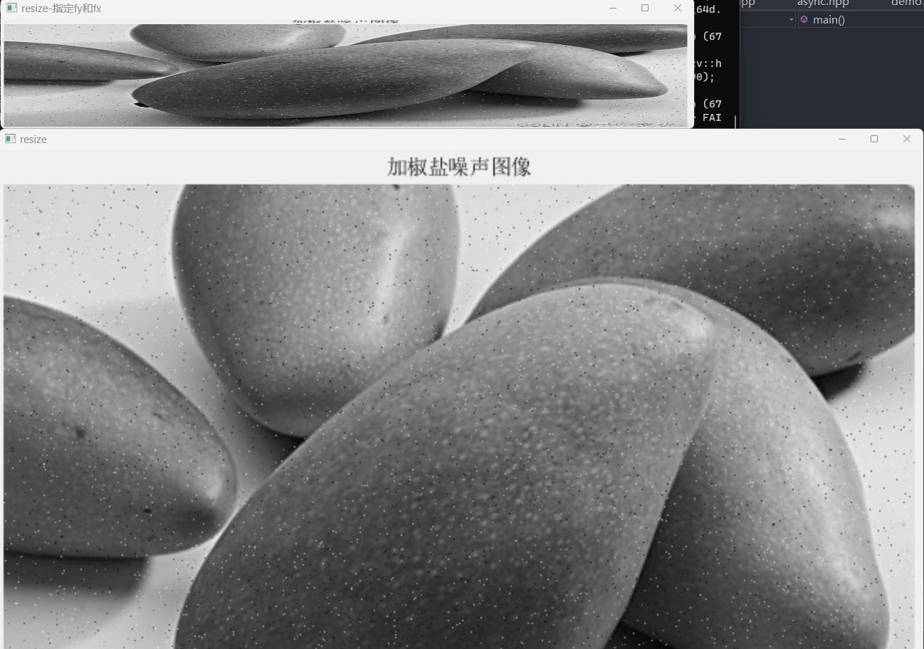
cv::resize(src, dst, src.size()*2);
imshow("resize", dst);
//指定fx和fy
cv::resize(src, dst, Size(), 1.5, 0.3);
imshow("resize-指定fy和fx", dst);
waitKey(0);
}
1.1.5.3. 阈值分割
- 固定阈值分割
Threshold@param src input array (multiple-channel, 8-bit or 32-bit floating point). @param dst output array of the same size and type and the same number of channels as src. @param thresh threshold value. @param maxval maximum value to use with the #THRESH_BINARY and #THRESH_BINARY_INV thresholding types. @param type thresholding type (see #ThresholdTypes). @return the computed threshold value if Otsu's or Triangle methods used. @sa adaptiveThreshold, findContours, compare, min, max */ CV_EXPORTS_W double threshold( InputArray src, OutputArray dst, double thresh, double maxval, int type );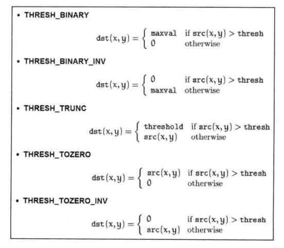
- 自适应阈值分割
adaptiveThreshold对矩阵采用自适应阈值操作,支持就地操作。
1.2. 图像变换
本章主要介绍的内容:
- 基于opencv的边缘检测
- 霍夫变换
- 重映射
- 仿射变换
- 直方图均衡化
1.2.1. 基于opencv的边缘检测
opencv中边缘检测有很多种算子和滤波器——Canny算子、Sobel算子、Laplacian算子以及Scharr滤波器
1.2.1.1. 边缘检测的一般步骤
- 滤波 边缘检测的算法主要是基于图像强度的一阶和二阶导数,但导数对噪声很敏感,因此必须采用滤波器来改善边缘检测器的性能。常见的滤波方法有高斯滤波、中值滤波等
- 增强 增强边缘的基础是确定图像各点邻域强度的变化值,增强算法可以将图像灰度点邻域强度值有显著变化的点凸显出来
- 检测
实际工程中,常用的方法是通过阈值化方法来检测,另外需要注意,Laplacian算子、Sobel算子和Scharr算子都是带方向的。
1.2.1.2. canny算子
John F.Canny于1986年开发的一个多级边缘检测算法,且Canny创立了边缘检测计算理论,解释了这项技术是如何工作的。Canny边缘检测算法被很多人推崇为当今最优的边缘检测算法。 最优边缘检测的三个主要评价标准:
- 低错误率:标识出尽可能多的实际边缘,尽可能减少噪声产生的误报
- 高定位性:标识出的边缘要与图像中的实际边缘尽可能接近
- 最小响应:图像中的边缘只能标识一次,并且可能存在的图像噪声不应标识为边缘
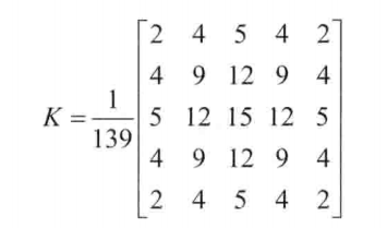
1.2.1.2.1. canny边缘检测的步骤
- 消除噪声
使用高斯平滑滤波器卷积降噪,以下是一个size=5的高斯内核示例:
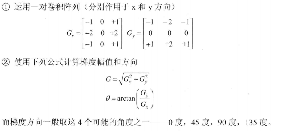
- 计算梯度幅值和方向
Canny边缘检测器使用了Sobel算子来计算梯度幅值,步骤如下:
- 非极大值抑制 这一步排除非边缘像素,仅仅保留了一些细线条(候选边缘)
- 滞后阈值
这是最后一步,canny使用了滞后阈值,滞后阈值需要两个阈值(高阈值和低阈值):
- 若某一像素位置的幅值超过高阈值,该像素被保留为边缘像素
- 若某一像素位置的幅值小于低阈值,该像素被排除
- 若某一像素位置的幅值在两个阈值之间,该像素仅仅在连接到高于高阈值的像素时被保留。
1.2.1.2.2. canny()函数
/** @brief Finds edges in an image using the Canny algorithm @cite Canny86 .

The function finds edges in the input image and marks them in the output map edges using the
Canny algorithm. The smallest value between threshold1 and threshold2 is used for edge linking. The
largest value is used to find initial segments of strong edges. See
<http://en.wikipedia.org/wiki/Canny_edge_detector>

@param image 8-bit input image.
@param edges output edge map; single channels 8-bit image, which has the same size as image .
@param threshold1 first threshold for the hysteresis procedure.
@param threshold2 second threshold for the hysteresis procedure.
@param apertureSize aperture size for the Sobel operator.
@param L2gradient a flag, indicating whether a more accurate \f$L_2\f$ norm
\f$=\sqrt{(dI/dx)^2 + (dI/dy)^2}\f$ should be used to calculate the image gradient magnitude (
L2gradient=true ), or whether the default \f$L_1\f$ norm \f$=|dI/dx|+|dI/dy|\f$ is enough (
L2gradient=false ).
 */
CV_EXPORTS_W void Canny( InputArray image, OutputArray edges,
                         double threshold1, double threshold2,
                         int apertureSize = 3, bool L2gradient = false );
参数详解:
- image:输入图像
- edges:输出的边缘图,需要和源图像有一样的尺寸和类型
- threshold1:第1个滞后性阈值
- threshold2:第2个滞后性阈值
- int apertureSize:表示Sobel算子的孔径大小,有默认值为3
- bool L2gradient:一个计算图像梯度幅值的表示,有默认值false 注意:threshold1和threshold2两者中较小的值用于边缘连接,较大值用来控制强边缘的初始段,推荐的高低阈值比为2:1到3:1之间。
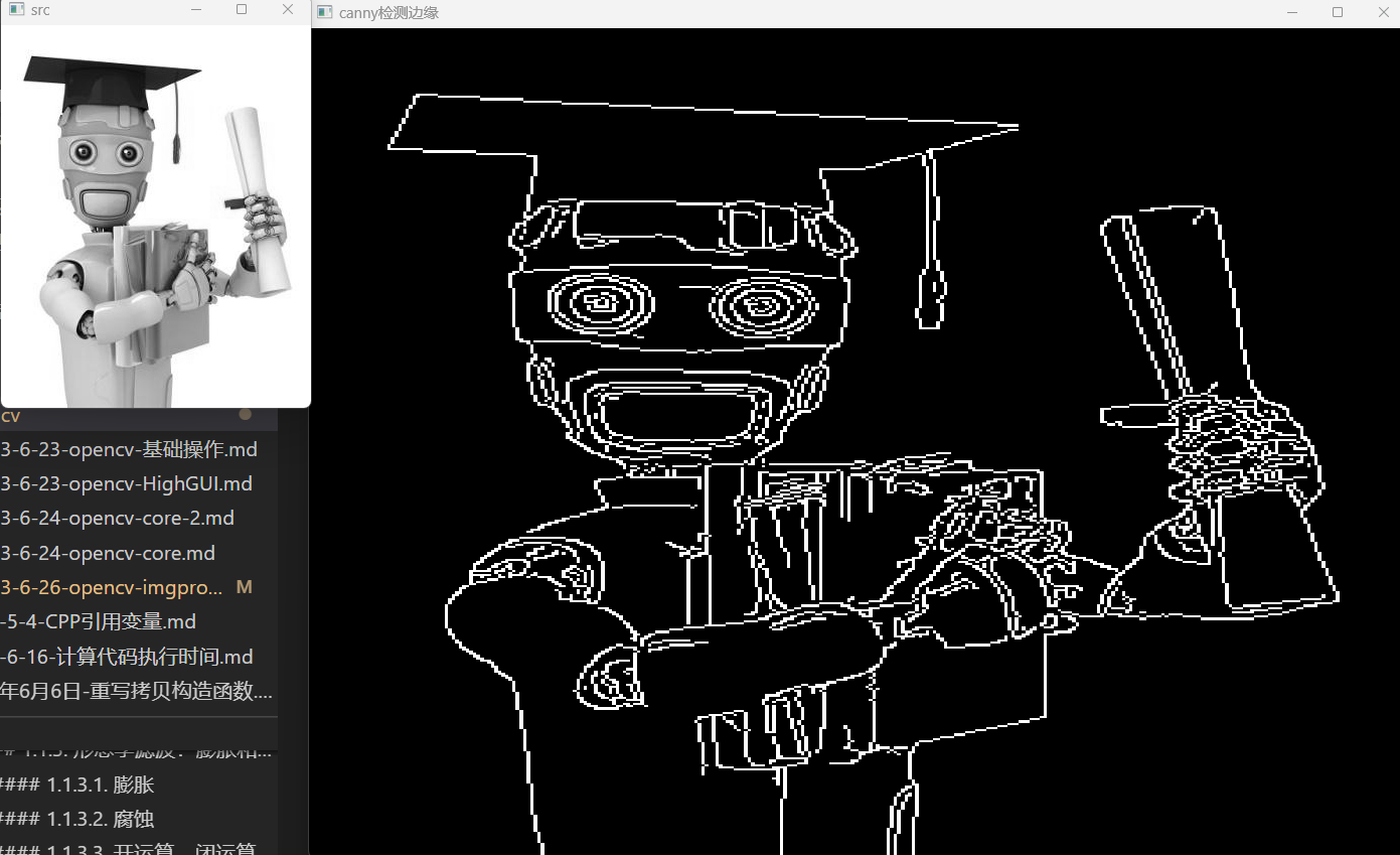
示例:
#include<opencv2/opencv.hpp>

using namespace cv;
int main()
{

	Mat src = imread("E:\\ml.png", IMREAD_GRAYSCALE);
	Mat edge;
	cv::Canny(src, edge, 50, 150);
	imshow("src",src);
	const char* wName = "canny检测边缘";
	namedWindow(wName, WindowFlags::WINDOW_NORMAL);
	imshow(wName, edge);
	waitKey(0);
}
效果:
1.2.2. 霍夫变换
霍夫变换实质上是特征空间的转换,通过变换特征空间,对特征进行投票来实现定位特征,常用来查找直线和圆形
1.2.2.1. 霍夫直线查找
参考:https://blog.51cto.com/u_15060531/4729201 https://zhuanlan.zhihu.com/p/203292567 https://blog.csdn.net/u013270326/article/details/73292076
1.2.2.1.1. 函数原型
opencv中通过HoughLines函数来基于霍夫变换找到直线
CV_EXPORTS_W void HoughLines( InputArray image, OutputArray lines,
                              double rho, double theta, int threshold,
                              double srn = 0, double stn = 0,
                              double min_theta = 0, double max_theta = CV_PI );
参数详解:
- InputArray image:输入图像
- OutputArray lines:输出直线的表示,是一个元素为Vec2f或Vec3f的vector,包含rho、theta或rho、theta、votes
- double rho:Distance resolution of the accumulator in pixels
- double theta:Angle resolution of the accumulator in radians.
- int threshold:threshold Accumulator threshold parameter. Only those lines are returned that get enough
- double srn:默认值0,对于multi-hough变换,distance resolution是rho/srn
- double stn: 默认值0,对于multi-hough变换,theta resolution是theta/stn
- double min_theta:直线的最小角度
- double max_theta: 直线的最大角度
1.2.2.1.2. 例子
#include<opencv2/opencv.hpp>

using namespace cv;
int main()
{
	Mat src=imread("E:\\shape.png");
	Mat midImage, dstImage;
	cv::Canny(src, midImage, 50, 200, 3);
	cv::cvtColor(midImage, dstImage, ColorConversionCodes::COLOR_GRAY2BGR);
	std::vector<cv::Vec2f> lines;
	//霍夫直线查找
	cv::HoughLines(midImage, lines, 1, CV_PI / 180, 150, 0, 0);
	for (size_t i = 0; i < lines.size(); i++)
	{
		float rho = lines[i][0], theta = lines[i][1];
		double a = cos(theta), b = sin(theta);
		Point p1, p2;
		double x0 = a * rho, y0 = b * rho;
		p1.x = cvRound(x0 + 1000 * (-b));
		p1.y = cvRound(y0 + 1000 * (a));
		p2.x = cvRound(x0 - 1000 * (-b));
		p2.y = cvRound(y0 - 1000 * (a));
		line(dstImage, p1, p2, Scalar(55, 100, 195), 1, LineTypes::LINE_AA);
	}

	imshow("src", src);
	imshow("边缘检测图", midImage);
	imshow("检测结果图", dstImage);
	waitKey(0);
}
效果:

1.2.2.2. 累计概率霍夫直线查找
/** @brief Finds line segments in a binary image using the probabilistic Hough transform.
The function implements the probabilistic Hough transform algorithm for line detection, described
in @cite Matas00
See the line detection example below:
@include snippets/imgproc_HoughLinesP.cpp
This is a sample picture the function parameters have been tuned for:

And this is the output of the above program in case of the probabilistic Hough transform:

@param image 8-bit, single-channel binary source image. The image may be modified by the function.
@param lines Output vector of lines. Each line is represented by a 4-element vector
\f$(x_1, y_1, x_2, y_2)\f$ , where \f$(x_1,y_1)\f$ and \f$(x_2, y_2)\f$ are the ending points of each detected
line segment.
@param rho Distance resolution of the accumulator in pixels.
@param theta Angle resolution of the accumulator in radians.
@param threshold Accumulator threshold parameter. Only those lines are returned that get enough
votes ( \f$>\texttt{threshold}\f$ ).
@param minLineLength Minimum line length. Line segments shorter than that are rejected.
@param maxLineGap Maximum allowed gap between points on the same line to link them.
@sa LineSegmentDetector
*/
CV_EXPORTS_W void HoughLinesP( InputArray image, OutputArray lines,
double rho, double theta, int threshold,
double minLineLength = 0, double maxLineGap = 0 );
1.2.3. 重映射-remap
g(x,y)=f(h(x,y)) 其中,g是目标图像,f是源图像,h(x,y)是映射函数,比如:对于图像I,h(x,y)=(I.cols-x,y)作为映射函数,结果就是目标图像是源图像关于y轴的对称图像